Users Manual

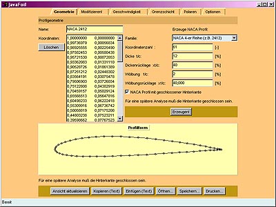
Geometry Card

It shows a list of coordinates and a plot of the resulting airfoil shape. You can enter or paste arbitrary coordinates into this field and press the "Update View" button to copy the coordinates into the working airfoil. Remember that the coordinates must be ordered trailing edge > upper > nose > lower > trailing edge.

Additionally it contains options to create standard airfoils from several families, namely:

• 4-digit series, like NACA 2415, based on
  • maximum thickness and its x/c location
  • maximum camber and its x/c location
• 5 digit series like NACA 23015, based on
  • maximum thickness and its x/c location
  • design lift coefficient
  • x/c location of maximum camber
• 16-series like NACA 16-412, based on
  • maximum thickness and its x/c location
  • design lift coefficient
• 6-series like NACA 64-412, based on
  • maximum thickness and its x/c location
  • design lift coefficient
  • camber line specification (a=...)
  • A-Modification
    Note that the 6-series sections are only approximated, for correct data use tables from NACA reports.

• TsAGI "B" series airfoils, based on
  • maximum thickness
• NPL "EC", "EH" series airfoils, based on
  • maximum thickness and its x/c location
  • maximum camber and its x/c location
• symmetrical Circular Arc airfoils, based on
  • maximum thickness
• symmetrical Double Wedge airfoils, based on
  • maximum thickness and its x/c location
• Cambered Plate airfoils, based on
  • maximum thickness
  • maximum camber and its x/c location
• Van de Vooren conformal mapping airfoil, based on
  • maximum thickness
  • trailing edge angle
• Newman airfoil, based on
  • maximum thickness
• Helmbold-Keine airfoil, based on
  • maximum thickness and its x/c location
  • trailing edge angel
  • radius at center of airfoil
  • leading edge radius
    Note that only a subset of possible parameters leads to reasonable shapes.

Note about all x-y graphs:

1. You can copy most of the graphs to the clipboard or save them to a file in AutoCad DXF, Adobe Illustrator encapsulated Postscript or SVG vector graphics format by pressing the right mouse button while the mouse pointer is located over the graph (context menu).
   Paste the test into a text editor, save as filename.dxf, .eps/.ai or .svg and import into your favorite graphics, CAD or word processing program.
2. If you have allowed the applet to write files, or if you run JavaFoil standalone, you can also export the graphics directly to a file, without using the clipboard.
3. Additionally, you can import numerical data into a graph to enhance it. For example you can import test results into the the polar plot for comparison. Import works only, if the graph already contains some data, so that the axis system is already set up. The data is lost when the graph is cleared for a new calculation, though.

You can save the generated coordinate set in several file formats. Note that JavaFoil recognizes the file type by its extension, so you have to stick to the proposed extensions.

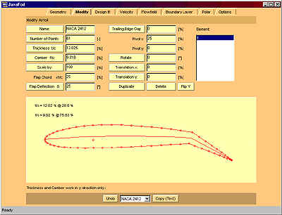
Modify Card

You can create a new distribution of points, change the camber and the thickness or deflect a plain flap. A scaling and rotating option is also available to transform the airfoil. The result of any modification is shown at the bottom of the card and is also transferred back to the Geometry card. Each transformation is executed when you press the button to the left of the corresponding text entry field.

Before a modification is performed JavaFoil saves a copy of the current geometry on top of a stack and you can either use the "Undo" button to back up to the previous configuration or select the desired configuration from the combo box. It is recommended to enter a name which reflects your modification before pushing the "Modify" button (e.g. "NACA 0010 / F+10" for a 10° flap deflection). To reduce memory overhead, the number of undo steps is currently limited to 10. Each additional modification will drop one saved geometry from the bottom of the stack.

Notes:

1. Changes to the camber are performed by scaling an existing camber line. Thus it is not possible to camber a symmetrical airfoil, as this would additionally require the specification of a camber line shape.
2. Changes act on the selected airfoil element(s) (in case of multi-element airfoils).

Changing the Number of Points

You can increase or decrease the number of points of the selected airfoil element. If you specify a negative number of points, JavaFoil uses a special tight spline curve which produces an almost linear interpolation between the given coordinate points.

 

Deflection of a simple Flap

Uses the given a flap chord and deflection angle (positive = trailing edge down) to rotate the coordinate points covered by the flap. No points are added to the convex side of the airfoil, so any initially coarse distribution might lead to a poor representation of the flapped airfoil. Also some points on the concave side are deleted if they would move inside of the flapped airfoil.

 

Modification of Thickness and Camber

Creates a new shape based on the camber distribution and the thickness distribution of the current airfoil. Both distributions are derived by analysis of the y-coordinates for a given x station - the thickness distribution is not applied at right angles to the camber line. This will introduce a small error where the camber line has a larger inclination. The extracted distributions are then scaled with the ratio of prescribed to current maximum value. The x-axis is defined to be the straight line from the trailing edge to the coordinate point having the largest distance to the trailing edge.

 

Scaling

Scaling is always performed with respect to the origin of the coordinate system (0/0). X and Y coordinates are multiplied with the given factor.

 

Trailing Edge Gap

The upper and lower surface of the airfoil are rotated around the leading edge point to open or close the trailing edge.

 

Rotation and Translation x/y

Allows arbitrary modifications to the position of the airfoil.

 

Duplicate

Creates a copy of the selected airfoil element. You have to move and/or rotate it afterwards so that it does not overlap its parent.

 

Delete

Deletes the selected airfoil element.

 

Flip Y

Mirrors the selected airfoil element along the x-axis (upside down transformation).

 

Copy (Text)

Copies a text buffer to the clipboard if your system security settings allow this. The buffer contains the coordinates of the camber distribution (x_c/y_c) and the coordinates of the thickness distribution (x_t/y_t) for the current airfoil.

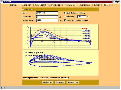
Design Card

Pressing the "Setup" button initializes the design procedure by copying the current airfoil. This airfoil is then analyzed at the given angle of attack and produces an initial target pressure distribution.

Now you can modify this pressure distribution either by using a smooth distortion of the target Cp or in a single point mode. Simply grab a point on the target distribution and drag it up or down to modify the curve.

After you are satisfied with the target Cp-distribution, you can run several design cycles and check the result. The current solution is overlaid on the previous results to allow for convergence check.

You can "Redraw" the screen to clear the intermediate results.

Instead of viewing the Cp-distribution in the usual way Cp=f(x/c) you can "unfold" the distribution by plotting Cp=f(s). Here s is the arc length measured along the airfoil surface (the order is upper surface, nose, lower surface). This representation makes it easier to modify the leading edge region.  When this viewing mode is active, a slider can be used to enlarge the leading edge or trailing edge regions.

A relaxation factor helps to stabilize the procedure and to smooth the geometry changes - usually a value between 10% and 25% is sufficient.

Typically, the number of design steps should be between 10 and 50 steps. You can repeat the design until JavaFoil has reached the target.

The analysis takes into account the effects of ground proximity as well as multiple elements. Note that the design procedure only acts on the first element of multiple elements. You have to change the order on the Geometry card if you want to design another element.

If you want to define the target pressure distribution by numbers, you can use the "Details..." button to open a window where you can enter or paste x/c, y/c, Cp triples. From these data, JavaFoil only reads the Cp values, changing x/c or y/c will have no effect.

Notes:

1. When "symmetric Cp modification" is checked, the Cp curves for upper and lower surfaces are modified in the same manner. This results in a global modification of the airfoil thickness.
2. When "anti-symmetric Cp modification" is checked, the Cp curves for upper and lower surfaces are modified with reversed signs. This results in a global modification of the airfoil camber.
3. When none of both options is checked, you can modify the Cp values for single points, which is useful for smoothing wavy airfoils.
4. The method is not foolproof and may diverge if the changes are too large. Problems may occur if modifications close to the leading and trailing edges are performed. This is because the stagnation point region is very sensitive to small changes in overall circulation.
5. The tool tries to translate any arbitrary Cp-distribution into a shape. If the target distribution is "ill posed", it may happen that no shape exists which creates such a distribution!
6. Markers on the airfoil shape indicate the results of the boundary layer analysis: green: transition, red: separation.

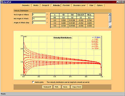
Velocity Card

The graph shows the velocity on both sides of the airfoil and can be used to smooth airfoils. If the velocity distributions show wiggles and zig-zag waves, any subsequent boundary layer analysis on the Polars card will probably create unrealistic results. To smooth an airfoil, go back to the Geometry card and change single y-coordinate values or use the Design card to modify the velocity distribution directly. Then re-analyze. Yes, this is slow, but possible and probably better than an automatic global smoother which would smooth over the whole airfoil.

You can display either the distribution of the local velocity v/V or the resulting local pressure coefficient C_p. If  a Mach number other than zero is specified on the Options card, the critical velocity ratio V* respectively the critical pressure coefficient C_p* is plotted also. The distributions are corrected for compressibility effects by the Karman-Tsien rule, but one must be aware of the fact that such corrections are valid only for Mach numbers below approximately 0.7.

Notes:

1. The Mach number from the Options card will be used for a compressibility correction on all cards. The corrections work reasonably well for Mach numbers below 0.75. If supersonic flow occurs somewhere on the airfoil surface, the code will not fail, but you would need a different type of analysis code for transonic and supersonic flow.
2. The table in the upper right of the card lists force and moment coefficients which are determined for the Reynolds number taken from the boundary layer card. However, the velocity distribution shown is for the inviscid flow. i.e. will not be affected by Reynolds number.
3. The table also shows the critical Mach number for each angle of attack. If the onset flow exceeds this Mach number, supersonic flow will occur somewhere on the airfoil. This Mach number is also known as the "Critical Mach number". As usual you can copy it using the context menu.

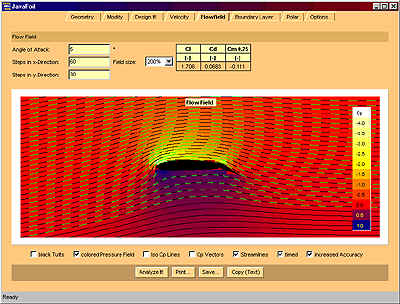
Flow Field Card

You can specify a regular x-y grid and an angle of attack. After solving for the surface velocity distribution, an evaluation is performed for each point on the grid. 

The buttons in the control bar at the bottom of the card perform the following actions:

Analyze It!

performs the analysis of the flow field at all grid points plus any additional post-processing like streamlines or iso-Cp lines.

 

Print...

Sends a copy of the picture to the printer, if your system security settings allow this.

 

Save...

Creates a text buffer which contains the coordinates and the velocity vector for each grid point (x, y, v_x,  v_y and v). This text buffer is saved to a file if your system security settings allow this. The format is suitable for the commercial plotting program Tecplot™ (by Amtec Corp.).

 

Copy (Text)

Like the Save... command, but the text buffer is copied to the clipboard if your system security settings allow this.

Notes:

1. As each evaluation can be time consuming, it is recommended to start with the coarse default grid and refine depending on the power of your computer and the amount of time you wish to spend. 
2. The rectangular grid is simply placed on top of the airfoil. It is not adapted to the airfoil shape. While interior points are excluded in the calculation, a coarse grid will create a rough outline of the airfoil only.
3. The graph shows, how the airfoil affects the whole flow field, not only the immediate neighborhood of the section.

• tufts ... shows a black "tuft" at each grid point, which is aligned with the local flow direction.
• colored cells ... colors a rectangle around each grid point according to the local pressure. This makes for a nice picture of the pressure field around the airfoil and shows how far the pressure is changed due to the airfoil.
• iso Cp ... plots lines of constant pressure, like altitude lines on a map.
• Cp-Vectors ... plots pressure vectors normal to the airfoil surface.
• stream lines ... black stream lines are drawn starting at the left border. The result resembles the injection of smoke into a wind tunnel.
• timed stream lines ... the stream lines are dashed to show the distance traveled during equal time intervals. Models something like a pulsed smoke generator. You will notice that particles arriving side by side at the leading edge will NOT meet again at the trailing edge.
• higher accuracy ... this option controls the calculation of the stream lines only. When selected, a 4th order Runge-Kutta scheme and a smaller time step are used, otherwise simple forward differencing is employed. The results are more accurate in regions where the streamlines are highly curved - calculation time is increased by a factor of 5, though.

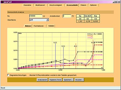
Boundary Layer Card

More details...

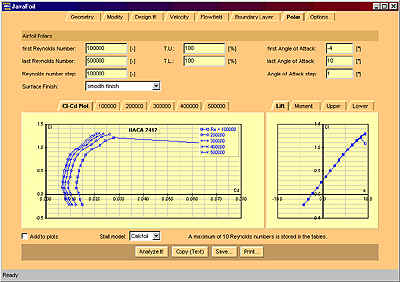
Polars Card

After specification of the desired Reynolds number and angle of attack range as well as selecting a surface roughness you can start the analysis. For each Reynolds number / angle of attack condition, JavaFoil will first calculate the velocity distribution and then perform a boundary layer analysis. The resulting lift, drag and moment coefficients as well as location of transition and separation will be presented in graphs and tables. A transition strip can be simulated by specifying a transition location x/c for both sides of the airfoil (the default setting of 100% corresponds to natural transition).

The user can select between different stall and transition models (the transition models are described here).

Note: It is not necessary to use the Velocity Card before calculating polars.

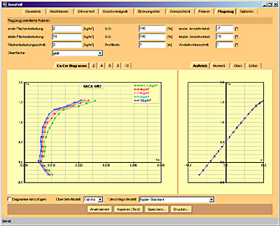
Aircraft Card

The Aircraft card makes it possible to analyze airfoils in an aircraft oriented way. It does not analyze and aircraft, though!

Instead of specifying a Reynolds number range you specify a range of wing loadings. Additionally you define the mean chord length and of course a range for the angle of attack. For each wing loading / angle of attack condition, JavaFoil will now find the matching Reynolds number. Like on the Polars card, the resulting lift, drag and moment coefficients as well as location of transition and separation will be presented in graphs and tables.

Note that the kinematic viscosity and the density are taken from the Options card. For different altuitudes you have to adjust these values accordingly.

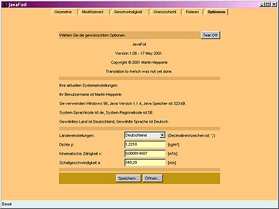
Options Card

You can save and restore the current state of JavaFoil to revert later to a previous project (see security settings).

Also you can specify some properties of the fluid where you want the airfoil to operate. The kinematic viscosity is needed for the calculation of the local Reynolds number and the speed of sound is needed for the Mach number. Currently, these parameters are currently only required for the Aircraft card.

The aspect ratio is used for an approximate correction of the results on the Polar and Aircraft cards for a finite wing. First the 3D lift coefficient C_L is determined by adapting the 2D C_l. Mach number and aspect ratio are taken into account. Then the 3D drag coefficient C_D is calculated by adding the induced drag coefficient for a wing with elliptical lift distribution to the C_d of the airfoil.

Finally, the scripting facility can be used to automate simple command sequences.